A spreadsheet addict shares his three favorite tips for marketers

I’m addicted to spreadsheets.  My friends know that I build spreadsheets for everything: I’ve got one for my to-do projects (Getting Things Done style).  One to manage my stock investing. And of course I’ve got one for this blog. In the world of data-driven marketing, spreadsheets let us do so much before we have to break out SQL and databases. The beauty of spreadsheets of course are the formulas - you can practically write a new operating system if you just make enough tabs! But far too often, I find myself “making do” with the formulas I already know instead of learning a faster, more specialized formula.  In fact, it was only this year that I finally got into the magic of Match Index formulas! So today, let me share some of my favorite spreadsheet formulas and shortcuts with you.

The Basic Bundle

I’m going to assume you already know how to use these three powerful formulas.  If not go look them up on ExcelJet.  Queries with these formulas might not always be pretty, but you can make them do almost anything you want. VLOOKUP Easy to pick up, but not quite as powerful as INDEX MATCH (see below). IF Fantastic little formula, but very quickly leads to bloated code. I still use one that’s 114 lines with 118 IF formulas. It works, but it’s not always the best option. SUMIFS Nothing too complicated but comes in handy more often than I’d think.

The Exciting Stuff

Ok, now lets get into the tricks that will change your life and turn you into a spreadsheet junkie like me. INDEX MATCH (to lookup anything)

=INDEX(data,MATCH(val,rows,1),MATCH(val,columns,1))

I put off learning INDEX MATCH for years because it seemed complicated.  Now I don’t know how I lived without it. Here’s how it works. Imagine you have a table tracking the number of dinosaur spottings each year in five cities: 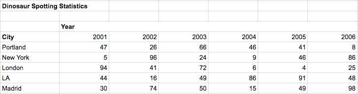From this table, you want to easily identify the number of spottings in New York in 2004. Or maybe in Portland in 2001. First, you want to identify the table area you’re searching:

=index(H6:M10

Second, you use a MATCH formula to tell it which row to identify. This simply says, “I want data from the row labeled ‘Portland’”.

=index(H6:M10,match("Portland",G6:G10,0)

Thirdly, use a second MATCH formula to identify the proper column. This just says, “I want data from the column labeled ‘2004’”.

=index(H6:M10,Match("Portland",G6:G10,0),match("2004",H5:M5,0))

Now you’ve got a very respectable query that will tell you Portland had 46 dinosaur spottings in 2004.  But what if you want to look up LA in 2006?  You’ll have to make changes to your hardcoded formula, and that’s not very fun. So let’s take it one step further. Instead of writing “Portland” and “2004” directly into the formula, let’s put those in separate cells and have the formula reference those cells:

=index(H6:M10,Match(H14,G6:G10,0),match(H15,H5:M5,0))

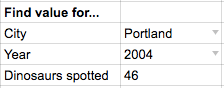Boom! Now you can change the city and year to anything you want, and your fancy new formula will dig through your table to find the right data. So the INDEX MATCH formula really isn’t that scary after all - just specify (1) the data range, (2) the row, and (3) the column. (See the formula live here.) “&” Operator (to join text fields)

=val&" "&val

Ok, here’s an even easier one. Imagine you have a list of customer names, but they’re split into two columns: first and last names.  How do you convert those two columns into one combined column? 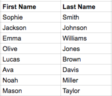Adding them together doesn’t work, and CONCATENATE gives unusable results (SophieSmith).  We need to combine the cells, but there should be a space between the words. This is where the magic of ampersand comes to the rescue.  Using “&” concatenates text strings and you can use two quotes around a space to add in the critical space:

=G3&" "&H3

Now just copy it down and you’ve got useable data: 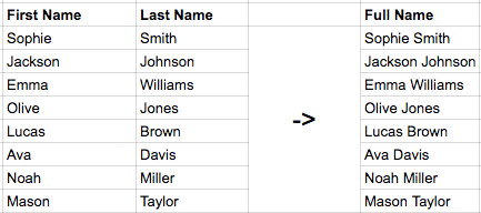And if you’ve got full names but need to split into first/last? Just use “text to column” to split on the space between words - it’s a tool available under the “Data” dropdown. (See the formula live here.) ”$” Operator (to create a static cell reference)

=FORMULA($column$row)

Spreadsheets are great because they let you create relative cell references. You reference cell A1, copy the formula down, and it automatically knows to adjust the reference in each row: A1, A2, A3, A4, etc.  Except sometimes you don’t want the reference to move with you. Say you’ve got a list of orders and you need to add your flat shipping fee to calculate totals due: 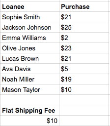So you create a formula that adds the purchase value to the flat shipping fee. You copy the formula down and nothing adds up.  The cell reference to $10 shipping fee moved with you and now you’re referencing blank cells. Thankfully there’s an easy fix: just add a “$” to make a row or column reference “locked”:

=H3+$G$13

Let’s break that down. See the “H3” reference? It’s looking at the contents of cell H3, but when we copy down a row it will automatically adjust to reference H4.  Now see ”$G$13” reference? you can copy it down, up, right, or left and that reference will continue pointing to cell G13. So now we can calculate purchase totals: 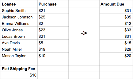And for bonus points, you can even be specific about locking column OR row.  In this case we’re copying the formula down, not over, so we just need to lock row movement: G$13 would work just fine.  However, $G13 wouldn’t work at all for this use case - that would lock column G, but still allow movement to row 14, 15, etc. (See the formula live here.)

The Biggest Spreadsheets Secret of All

As much fun as spreadsheets are, they can be overused.  Just because you can build a massive 3MB spreadsheet doesn’t mean you should - learning SQL will help you manage that level of data much more effectively.  And if you think the power of spreadsheets is fun, just wait ‘til you see what SQL can do!